Quantitative Hyperbolicity Estimates in One-Dimensional Dynamics

This page contains additional information and data referred to in the paper Quantitative hyperbolicity estimates in one-dimensional dynamics by Sarah Day, Hiroshi Kokubu, Stefano Luzzatto, Konstantin Mischaikow, Hiroe Oka, and Paweł Pilarczyk

Files for Download

Below is a list of files for download (please, see the description in the next sections). The zipped files should be uncompressed to empty subdirectories (folders), except for capd-capdDynSys-4.2.153.zip, which already includes a subfolder. Please, note that in Windows these files should be unzipped in the text mode to ensure the correct conversion of line endings (add the -a command-line switch in case of unzipping with the Info-ZIP software).

• unifexp-src.zip – source code of the software (updated),
• unifexp-dox.zip – documentation of the software (updated),
• unifexp-dat.zip – raw data files,
• capd-capdDynSys-4.2.153.zip – source code of the entire CAPD-DynSys subproject of the CAPD library, copied from the CAPD download site (compatible with the updated version),
• chomp-lib.zip – source code of part of the CHomP software library (compatible with the updated version).

• unifexp-src.zip – source code of the software (original version),
• unifexp-dox.zip – documentation of the software (original version),
• capd_src.zip – source code of the entire CAPD library (old version),
• chomp-full.zip – source code of the entire CHomP library (old version).

Software

The software for computations described in the paper is written in the C++ programming language for optimal effectiveness and flexibility. Detailed documentation of the software has been prepared with Doxygen. Feel free to browse this documentation and learn about the details of how the software was programmed. The file unifexp-dox.zip contains the compressed version of this documentation which is available here for easy download for off-line browsing; please, unzip the contents of the archive into an empty directory, and open the file index.html.

The file unifexp-src.zip containing the source code of the software is available here for download under the terms of the GNU General Public License. It is prepared for the compilation with the GNU C++ compiler, either in GNU/Linux (or a similar system), or in Windows in the MSYS environment. A relatively recent version of the compiler is required to compile the code correctly. The provided makefile must be adjusted before the compilation, especially as far as the paths to the CAPD and CHomoP libraries are concerned (please, see the explanations in the file itself).

The software uses the Boost, CHomP and CAPD libraries which are publically available, the last two under the terms of the GNU General Public License. Please, refer to the websites of those libraries for the source code and compilation instructions. Note that the Boost library is often included in standard GNU/Linux distributions, so no installation might be necessary. This is not the case with the other libraries, though. Even worse, since those libraries are undergoing dynamic development, it may turn out that their interface may slightly change in the future versions, so a copy of compatible versions of both libraries is available for download from this page (please, see the previous section).

Compilation of the Software

Step 1. Compilation of CHomP. This is my suggestion:

1. mkdir chomp
2. cd chomp
3. unzip -a ../chomp-lib.zip
4. make library
5. cd ..

Step 2. Compilation of CAPD. Since this library has many options, here is my suggestion for how to compile it. Note that it may be necessary to install the additional package pkg-config if it is not present in the system.

1. unzip -a capd-capdDynSys-4.2.153.zip
2. mkdir capd4
3. mkdir capd4_compil
4. cd capd4_compil
5. ../capd-capdDynSys-4.2.153/configure --prefix /home/your-dir/capd4 --with-filib=yes --with-mpfr=no --with-boost=/usr --without-gui
6. make
7. make install

Step 3. Compilation of the unifexp program. After having successfully compiled the CHomP and CAPD libraries, this is my suggestion how to proceed:

1. mkdir unifexp
2. cd unifexp
3. unzip -a ../unifexp-src.zip
4. make

Step 4. Testing the program. You can run a test computation to see if the program works:

• ./unifexp -p uniform -i --rigorous -k5001 -a1.83139961 -a1.83139961 --lambda --delta -L0 -L0 -f a00.dat --log a00.log --debug

Remark. It seems that the program unifexp does not compile with gcc 4.4.6 20120305 (Red Hat 4.4.6-4) due to a problem with the power function in CAPD. The same with gcc (Debian 4.4.5-8) 4.4.5. If you encounter this kind of a problem, please, try using a more recent version of the GCC compiler.

Remark for Mac users. I tested this software on a Mac with OS X El Capitan Version 10.11.6 and GNU C++ compiler 7.2.0 provided by MacPorts. For compiling the CHomP library, I used the command

• make target=macports

• export CC=gcc-mp-7 -m64
• export CXX=g++-mp-7 -m64
• ../capd-capdDynSys-4.2.153/configure --prefix /Users/pawel.pilarczyk/capd4 --with-filib=yes --with-mpfr=no --with-boost=/usr --without-gui CXX="g++-mp-7 -m64" CC="gcc-mp-7 -m64" CXXFLAGS="-O2 -Wall"

• make cxx="g++-mp-7 -m64"

Results of Computations

The raw data with the results of computations used to create the figures published in the paper, and also with some other results, can be downloaded below. All these results were produced by the software described in the previous section and are encoded in text files whose lines contain the following items as a space-separated list:

• the asterisk that indicates the beginning of a data set (comments are preceded with the semicolon)
• the identifier of the data piece in the format level:number (e.g., 4:12)
• the left end of the parameter interval (minimal parameter value)
• the right end of the parameter interval (maximal parameter value)
• the total number of intervals that cover both Δ and the remainder of I
• the diameter δ of the critical neighborhood
• the computed expansion exponent λ
• the computed value of log C (0 if not computed)
• the computed value of λ₀ (0 if not computed)
• the computation time measured in seconds

specifications	graphs
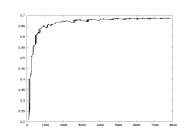
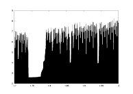
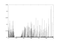
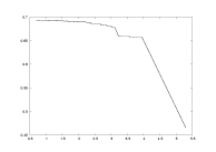
a01.dat   K=5000 delta: 0.005-0.5 a=2.0	lambda as a function of -log(delta)	computation time as a function of -log(delta)
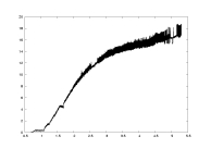
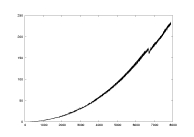
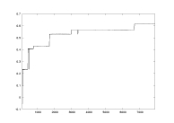
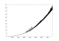
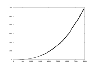
a02.dat   K: 100-7900 delta=0.01 a=2.0 Floyd-Warshall	lambda as a function of K	computation time as a function of K
a03.dat   K: 100-7900 delta=0.01 a=2.0 Johnson	lambda as a function of K	computation time as a function of K
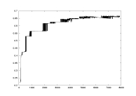
a04.dat   K: 100-7900 delta=0.01 a=2.0 critical partition	lambda as a function of K	comparison of lambda computed with critical vs. uniform partition
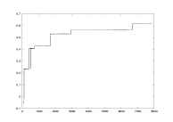
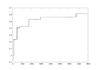
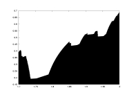
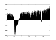
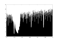
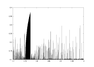
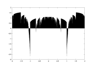
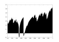
a05.dat   K=5000 delta=0.1 a: 1.7-2.0 critical partition	lambda as a function of a	lambda0 as a function of a
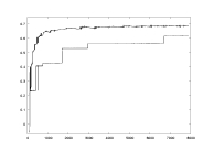
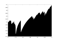
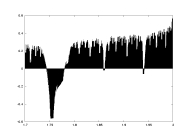
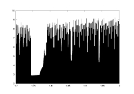
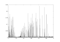
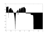
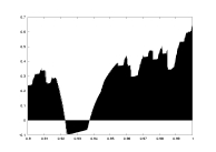
a06.dat   K=5000 delta=0.1 a: 1.7-2.0 uniform partition	lambda as a function of a	lambda0 as a function of a
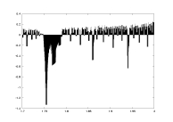
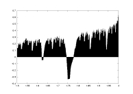
a07.dat   K=5000 delta=0.1 a: 1.7-2.0 derivative partition	lambda as a function of a	lambda0 as a function of a
a08.dat   K=5000 delta=0.001 a: 1.7-2.0	lambda as a function of a	computation time as a function of a
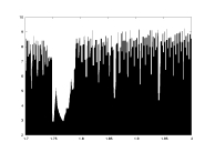
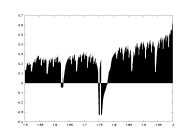
a09.dat   K=5000 delta=0.01 a: 1.7-2.0	lambda as a function of a	lambda0 as a function of a
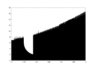
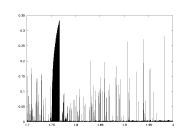
a10.dat   K=5000 delta min lambda>0 a: 1.7-2.0	-log(delta) as a function of a	lambda as a function of a
a11.dat   K=5000 delta min lambda>0.1 a: 1.7-2.0	-log(delta) as a function of a	lambda as a function of a
a12.dat   K=5000 delta min lambda0>0 a: 1.7-2.0	-log(delta) as a function of a	lambda0 as a function of a
a13.dat   K=5000 delta min lambda0>0.1 a: 1.7-2.0	-log(delta) as a function of a	lambda0 as a function of a
a14.dat   K: 100-7900 delta=0.01 a=2.0 (computing lambda only)	lambda as a function of K	computation time as a function of K
a15.dat   K=5000 delta=0.01 a: -2.0-2.0 cubic map non-rigorous	lambda as a function of a	lambda0 as a function of a
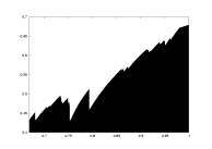
a16.dat   K=5000 delta=0.05 a: 0.67-1.0 unimodal map with gamma=1.5 non-rigorous	lambda as a function of a	lambda0 as a function of a
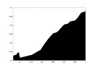
a17.dat   K=5000 delta=0.05 a: 0.9-1.0 unimodal map with gamma=2.5 non-rigorous	lambda as a function of a	lambda0 as a function of a
a18.dat   K=4000 delta=0.02 a: 1.5-2.0	lambda as a function of a	lambda0 as a function of a
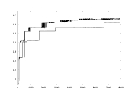
a19.dat   K: 100-7900 delta=0.01 a=2.0 derivative partition	lambda as a function of K	comparison of lambda computed with derivative vs. uniform partition

The figures in the paper were generated using the following data:

• Figure 3 - a01.dat
• Figure 4 - a02.dat
• Figure 5 - a02.dat and a04.dat
• Figure 6 - a02.dat and a03.dat
• Figure 7 - a10.dat
• Figure 8 - a09.dat
• Figure 9 - a10.dat

All trademarks, registered trademarks or brand names are property of the respective holders and used in this document for descriptive purposes only. Copyright © 2005-2024 by Paweł Pilarczyk. All rights reserved.