A stage-structured discrete population model with harvesting.
Results of computations

This website contains additional interactive information and raw data referred to in the paper Global dynamics in a stage-structured discrete population model with harvesting by Eduardo Liz and Paweł Pilarczyk, published in Journal of Theoretical Biology, Vol. 297 (2012), pp. 148-165.

These computations were done for the following 2-dimensional system:

A_n+1 = (1 – h_j) s_j J_n + (1 – h_a) s_a A_n
J_n+1 = g ((1 – h_a) A_n)
with the Ricker map g (x) = α x e^–βx

where A_n, J_n – the amounts of adults and juveniles in the n-th generation,

with the following meaning of the parameters:

h_a, h_j – harvesting rates for adults and juveniles, respectively
s_a, s_j – survival rates of adults and juveniles, respectively
α = e^r – parameter affecting the dynamics; fixed for r := 4
β – phase space scaling parameter; fixed as β := α / e

Continuation diagrams

Continuation diagrams for the six cases under consideration were computed as described in the paper, using an updated version of the Conley-Morse Graphs software (available from the author upon request).

The parameter space [0,1] x [0,1] was sampled at 500 x 500.
The phase space [0,1.35] x [0,1.35] was sampled at 1024 x 1024.

Each continuation diagram shows the respective harvesting rate in the horizontal axis, and the survival rate in the vertical axis.

The CPU time information is provided for a Quad-Core AMD Opteron™ Processor 2376 2.3 GHz (ca. 4600 bogomips). Memory usage information is approximate and was measured for the program compiled for the amd64 architecture with the GNU C++ 4.1.2 compiler.

The phase space shows the adult population size (A_n) in the horizontal axis, and the juvenile population size (J_n) in the vertical axis.

Each clickable diagram that loads when the corresponding link is clicked, allows to browse the results of computations by individual parameter boxes. An extra large version is provided to allow clicking parameter boxes more precisely, e.g., in order to check very small continuation classes.

[clickable diagram] [extra large version]	Case Ha–S1 hj = 0, sj = 1 – sa varying parameters: ha, sa 2,929 hours of CPU time 1,767 MB memory max	[clickable diagram] [extra large version]	Case Ha–Se hj = 0, sj = sa varying parameters: ha, sa 2,533 hours of CPU time 1,345 MB memory max
[clickable diagram] [extra large version]	Case Hj–S1 ha = 0, sj = 1 – sa varying parameters: hj, sa 1,410 hours of CPU time 607 MB memory max	[clickable diagram] [extra large version]	Case Hj–Se ha = 0, sj = sa varying parameters: hj, sa 1,115 hours of CPU time 220 MB memory max
[clickable diagram] [extra large version]	Case He–S1 hj = ha, sj = 1 – sa varying parameters: ha, sa 1,349 hours of CPU time 780 MB memory max	[clickable diagram] [extra large version]	Case He–Se hj = ha, sj = sa varying parameters: ha, sa 1,169 hours of CPU time 405 MB memory max

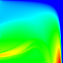
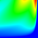
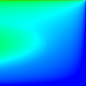
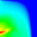
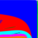
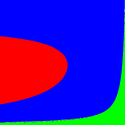
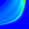
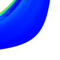
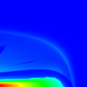
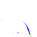
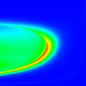
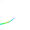
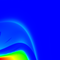
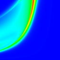
Averaged hydra effect analysis

Case Ha–S1			Case Ha–Se
[adult population size] 0.000659 – 0.999976	[hydra effect] 10% – 96.5546%		[adult population size] 0.000659 – 1.04946	[hydra effect] 10% – 212.76%
Case Hj–S1			Case Hj–Se
[adult population size] 0.000659 – 0.80079	[hydra effect] 10% – 25.8165%		[adult population size] 0.000659 – 0.917618	[hydra effect] (all below 10%)
Case He–S1			Case He–Se
[adult population size] 0.000659 – 0.801662	[hydra effect] 10% – 37.7829%		[adult population size] 0.000659 – 0.892547	[hydra effect] 10% – 45.9739%

Linear color scale from the lowest values (blue) to the highest ones (red).

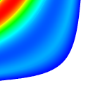
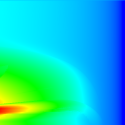
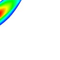
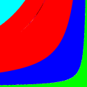
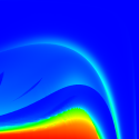
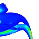
Numerical bubble effect analysis

Case Ha–S1			Case Ha–Se
[attractor size] 1 – 610,743	[bubble effect] 100% – 6,141.26%		[attractor size] 1 – 326,395	[bubble effect] 100% – 8,931.06%
Case Hj–S1			Case Hj–Se
[attractor size] 55 – 607,621	[bubble effect] 100% – 2,005.25%		[attractor size] 14 – 69,171	[bubble effect] 100% – 145.042%
Case He–S1			Case He–Se
[attractor size] 1 – 610,743	[bubble effect] 100% – 5,234.5%		[attractor size] 1 – 132,579	[bubble effect] 100% – 62,601%

Linear color scale from the lowest values (blue) to the highest ones (red).

All trademarks, registered trademarks or brand names are property of the respective holders and used in this document for descriptive purposes only. Copyright © 2005-2024 by Paweł Pilarczyk. All rights reserved.